VLSI DESIGN - Set Timing Derate

Timing Derate

In VLSI design, timing derate is a technique used to account for the variations in the timing of the circuit.

Timing derate scales nominal delays to model real‑world uncertainty such as process, voltage, temperature (PVT) variation and on‑chip variation (OCV). Instead of relying on a single “typical” delay, Static Timing Analysis (STA) applies multiplicative derate factors to cell and interconnect delays (and sometimes slews), creating pessimistic or optimistic views as needed for setup and hold checks.

Timing Derate Categories

Practically, tools use different derate categories:

• Early/Late derates (OCV): constant factors applied to model fastest/slowest cases.
• AOCV (advanced OCV): depth‑ and distance‑dependent tables that reduce over‑pessimism on short paths but retain safety on deep paths.
• POCV/SOCV (parametric/statistical OCV): sigma‑based models that capture correlated variation statistically, often yielding tighter yet safe margins.

Purpose and function in STA:

• Ensure setup safety: data path delays are derated “late” (scaled up) and launch clock “early” (scaled down) while capture clock is “late,” creating a worst‑case window for maximum path delay.
• Ensure hold safety: data path delays are derated “early” (scaled down) and launch clock “late” while capture clock is “early,” creating a worst‑case window for minimum path delay.
• Balance pessimism vs. realism: advanced models (AOCV/POCV) remove excessive guardband while maintaining sign‑off safety, improving achievable frequency and reducing unnecessary fixes.

Derates can be applied separately to cell vs. net, data vs. clock, and launch vs. capture legs, which is essential for accurate slack calculation under correlated and uncorrelated variation sources. Typical constant OCV factors might be, for example, 0.95 (early) and 1.05 (late) for cells, with slightly different values for nets; advanced flows replace constants with tables or statistical parameters.

Examples

Constant OCV example

Suppose a nominal data path delay is 500 ps (cell 350 ps + net 150 ps). With early/late derates of 0.95/1.05 for cells and 0.97/1.03 for nets:

• Setup (late data): max data delay ≈ 350×1.05 + 150×1.03 = 366 + 154.5 = 520.5 ps.
• Hold (early data): min data delay ≈ 350×0.95 + 150×0.97 = 332.5 + 145.5 = 478 ps.

These scaled delays are then used in the slack equations below along with appropriately derated launch/capture clock paths to stress worst‑case windows.

Now let’s see a PrimeTime example to set the derates:

# Data path derates
set_timing_derate -cell_delay -data -early 0.95
set_timing_derate -cell_delay -data -late  1.05
set_timing_derate -net_delay  -data -early 0.97
set_timing_derate -net_delay  -data -late  1.03

# Clock path derates (often slightly different; example shown)
set_timing_derate -cell_delay -clock -early 0.95
set_timing_derate -cell_delay -clock -late  1.05
set_timing_derate -net_delay  -clock -early 0.97
set_timing_derate -net_delay  -clock -late  1.03

# Optional: scope by mode/corner or hierarchy using -from/-to/-cells/-nets as needed

AOCV example

Path‑depth dependent derates reduce pessimism on short paths while keeping safety on deep paths. Example table (illustrative): | Depth | Cell Early | Cell Late | Net Early | Net Late | |—|—|—|—|—| | 1 | 0.93 | 1.07 | 0.96 | 1.04 | | 3 | 0.95 | 1.05 | 0.97 | 1.03 | | 6 | 0.97 | 1.03 | 0.985 | 1.02 |

For a depth‑3 path using the table above, use the row for 3 to scale the nominal cell/net components for setup/hold views. In practice, production flows source AOCV tables from libraries or sign‑off kits and the STA tool automatically picks the derate from the appropriate depth/distance bin per arc.

Simplified POCV/SOCV example

POCV models delay as a distribution with mean (μ) and standard deviation (σ). STA computes guardbanded delay using a sigma multiplier k that reflects the target yield and correlation.

• Setup worst‑case: delay ≈ μ + k·σ (e.g., k = +3)
• Hold worst‑case: delay ≈ μ − k·σ (e.g., k = +3)

Numeric example: if a path has μ = 500 ps and σ = 20 ps, then setup uses ≈ 500 + 3·20 = 560 ps; hold uses ≈ 500 − 3·20 = 440 ps. POCV reduces over‑pessimism by accounting for correlation across cells/nets, often yielding tighter yet still safe margins versus constant OCV.

Practical Examples

Given the following circuit diagram, let’s calculate the setup and hold slacks without and with derates. Suppose $T_{setup_chk}$ is 2ns and $T_{hold_chk}$ is 1ns.

The SDC constraints are as follows:

create_clock -name CLK -waveform {0 12} -period 20 [get_ports CLK]; # Period is 20ns with 12ns high and 8ns low

set_clock_uncertainty 2 -setup [get_clocks CLK]
set_clock_uncertainty 1 -hold  [get_clocks CLK]

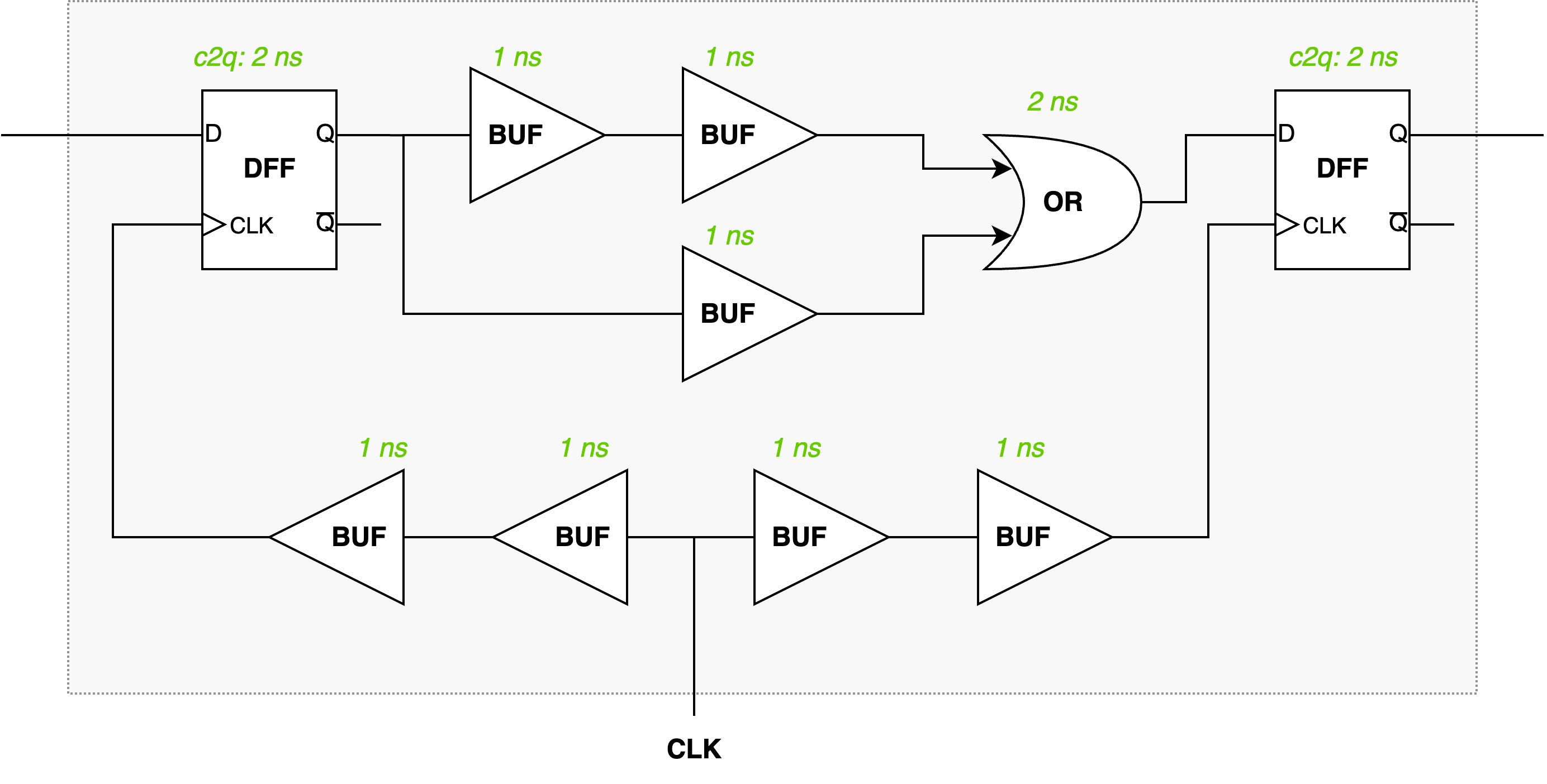
Without derates

The setup slack is calculated as follows:

\[\begin{align} T_{setup\_slack} &= T_{clk} + T_{clk\_capture} - T_{clk\_launch} - T_{comb\_path(max)} - T_{c2q} - T_{setup\_uncertainity} - T_{setup\_chk} \\ &= 20 + 2 - 2 - 4 - 2 - 2 - 2 \\ &= 10 ns \end{align}\]

The hold slack is calculated as follows:

\[\begin{align} T_{hold\_slack} &= T_{clk\_launch} + T_{comb\_path(min)} + T_{c2q} - T_{clk\_capture} - T_{hold\_uncertainity} - T_{hold\_chk} \\ &= 2 + 3 + 2 - 2 - 1 - 1 \\ &= 3 ns \end{align}\]

With derates

Now add the derates to the circuit diagram:

set_timing_derate 1.2 -late  -clock
set_timing_derate 1.1 -late  -data
set_timing_derate 0.9 -early -clock
set_timing_derate 0.8 -early -data

The setup slack will be:

\[\begin{align} T_{setup\_slack} &= T_{clk} + Td_{clk\_capture} - Td_{clk\_launch} - Td_{comb\_path(max)} - Td_{c2q} - T_{setup\_uncertainity} - T_{setup\_chk} \\ &= 20 + 2 * 0.9 - 2 * 1.2 - 4 * 1.1- 2 * 1.1 - 2 - 2 \\ &= 8.8 ns \end{align}\]

The hold slack will be:

\[\begin{align} T_{hold\_slack} &= Td_{clk\_launch} + Td_{comb\_path(min)} + Td_{c2q} - Td_{clk\_capture} - T_{hold\_uncertainity} - T_{hold\_chk} \\ &= 2 * 0.9 + 3 * 0.8 + 2 * 0.8 - 2 * 1.2 - 1 - 1 \\ &= 1.4 ns \end{align}\]

Extended Example

Now, let’s consider applying the same derates to a modified circuit where the buffer near the output DFF is replaced with an inverter. The updated circuit diagram is shown below:

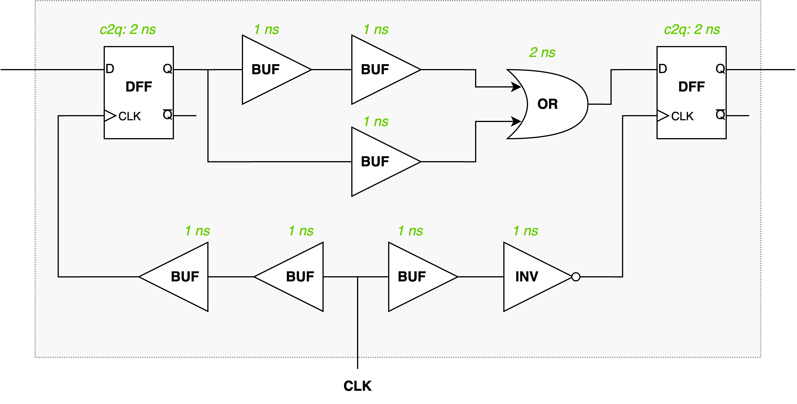
Since now the capture clock is 8ns in advance, the setup slack will be:

\[\begin{align} T_{setup\_slack} &= T_{cap\_shift} + Td_{clk\_capture} - Td_{clk\_launch} - Td_{comb\_path(max)} - Td_{c2q} - T_{setup\_uncertainity} - T_{setup\_chk} \\ &= 12 + 2 * 0.9 - 2 * 1.2 - 4 * 1.1- 2 * 1.1 - 2 - 2 \\ &= 0.8ns \end{align}\]

The hold check will not be performed at the same clock edge, so the hold slack will be:

\[\begin{align} T_{hold\_slack} &= (Td_{clk\_launch} + T_{lc\_shift}) + Td_{comb\_path(min)} + Td_{c2q} - (Td_{clk\_capture} + T_{cap\_shift}) - T_{hold\_uncertainity} - T_{hold\_chk} \\ &= (2 * 0.9 + 20) + 3 * 0.8 + 2 * 0.8 - (2 * 1.2 + 12) - 1 - 1 \\ &= 9.4 ns \end{align}\]

Is this blog helpful? Help fuel more in-depth technical content by treating me to a coffee! Your support keeps the knowledge flowing ☕✨